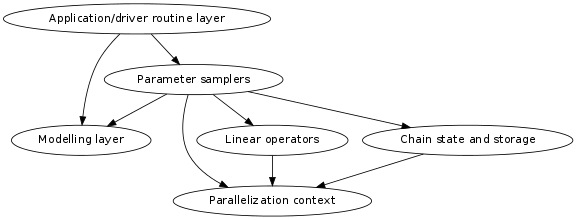
Architecture

Various aspects of Commander, ordered roughly from high-level to low-level layers.

A design goal of Commander is that the lower-level layers should be useful in their own right without involving the abstractions in the higher layers in any way.

This illustration is not finished:

Application/driver routine layer

The package commander.apps contain command-line applications and utilities. The most basic of these can be used directly, and are also available through scripts in /bin.

However, some applications require much more configuration than what can be conveyed on the command-line. In these cases, one calls the application routines while passing in something from the modelling layer which effectively acts as configuration (described below). Assuming [V1, V2] and [cmb, synchrotron, <...>] are objects from the modelling layer, one might invoke the CMB Gibbs sampler like this:

cm.apps.cmb_gibbs_sampler_command_line(
    observations=[V1, V2],
    signal_components=[cmb, synchrotron, free_free, monodipole],
    # <snip more options>
    chain_count=10,
    sample_count=5000,
    output_filename='wmap-9r-analysis.h5'
)

These application routines typically have two versions: One with and one without a ...command_line suffix. The command_line version will in addition to the provided options parse sys.argv for additional options, and in general provide more defaults.

Full example: See scripts/wmap_gibbs_sampler_runner.py.

Modelling layer

This layer is the primary API to set up the problem that Commander should solve. The objects are all entirely descriptive and take few or no actions on their own. An example:

V1 = cm.SkyObservation(
    name='V1',
    T_map=('$WMAPPATH/wmap_da_imap_r9_7yr_V1_v4.fits', 1, 'TEMPERATURE'),
    ...
    )
cmb = cm.IsotropicGaussianCmbComponent(
    power_spectrum='$WMAPPATH/wmap_lcdm_sz_lens_wmap7_cl_v4.dat',
    lmax=1500)
synchrotron = cm.SynchrotronComponent(nu_ref=60, lmax=1500)

Here, V1 and cmb are descriptors, their role is to carry around information/configuration, not to do anything. The constructors will resolve the filenames to absolute paths (so that a later os.chdir does not alter the contents), but no attempt is made to load any data.

While the constructor is not allowed to do anything intensive, model objects are allowed to provide methods that do loading or computation. The loading/computation will typically depend on the parallelization and so require a CommanderContext. E.g.:

ctx = cm.CommanderContext(my_mpi_communicator)

# load single map
map = V1.load_map(ctx)
# load many maps in parallel, more efficient
map_lst, rms_lst, mask_lst = cm.load_map_rms_mask(ctx, [V1, V2])

# Constructing the mixing operator of synchrotron requires some
# computation (integrating over the bandpass of the observation several times
# and compute a spline)
M_V1_sync = synchrotron.get_mixing_operator_sh(ctx, V1, beta=-2.2, C=2.12)

MCMC chains

The Chain and MemoryChainStore / HDF5ChainStore` classes cooperate to provide the abstractions for running an MCMC/Gibbs chain. They don’t do any sampling by themselves, but primarily allow a) persistence of chain, and b) passing around information about current chain state. By using these classes the boilerplate is greatly reduced from a typical MCMC loop, while still allowing for programming the chain in the good old imperative manner. See Chain documentation (TODO).

Linear operators

Commander uses the oomatrix library to deal with linear algebra. The library allows for plugging in your own linear operators, and many such operators have to be provided by Commander, e.g., spherical harmonic transforms and efficient component mixing. See scripts/simple_constrained_realization.py for an example of constrained realization being quickly implemented using only the linear operators.

Parallelization context

The CommanderContext (typically named ctx in code) is responsible for storing the parallelization scheme (and provide good defaults), and is conventionally passed as the first argument to many routines. Parallelization is coordinated by passing around the CommanderContext object. E.g., in the following code, it is assumed that the call is done collectively with the same arguments, and after the call map only contains the rings of the local rank:

map = cm.load_map(ctx, V1)

Note that it is not allowed to alter the arguments to load different bands on each rank:

map = cm.load_map(ctx, observations[comm.Get_rank()])

Rather, it is the responsibility of the CommanderContext to coordinate which map lives where:

# THIS WAY OF PARTITIONING IS NOT IMPLEMENTED, and may not be, the
# point is just for now to provide an example of the
# responsibilities of CommanderContext
ctx = CommanderContext(comm=comm_with_two_ranks,
                       observations=[V1, V2],
                       partition_by_observation=True)
map_lst, rms_lst, mask_lst = cm.load_map_rms_mask(ctx, [V1, V2])
# Now, rank 0 contains all V1 data and rank 1 contains all V2 data